
Incomplete.
How four identical numbers can hide four completely different decisions - and a Claude exercise to see it for yourself.

The numbers were identical. That was the problem.
Average click-through rate: 3.1%.
Average conversion rate: 4.3%.
Different audience segments, same summary stats, nothing alarming.
So the report went out, the strategy held, and nobody asked what was underneath.
Underneath:
One segment converting at 14%.
The other at less than 1%.
The “average” was blending completely different response patterns into one tidy number. The budget that looked balanced was simultaneously underinvesting in what was working and burning spend on what wasn’t.
The numbers weren’t wrong. They were incomplete. And “statistically identical” doesn’t mean “decision-wise the same.”
There’s a name for this class of problem.
It’s called Anscombe’s Quartet - four datasets that share identical summary statistics but look completely different the moment you plot them.
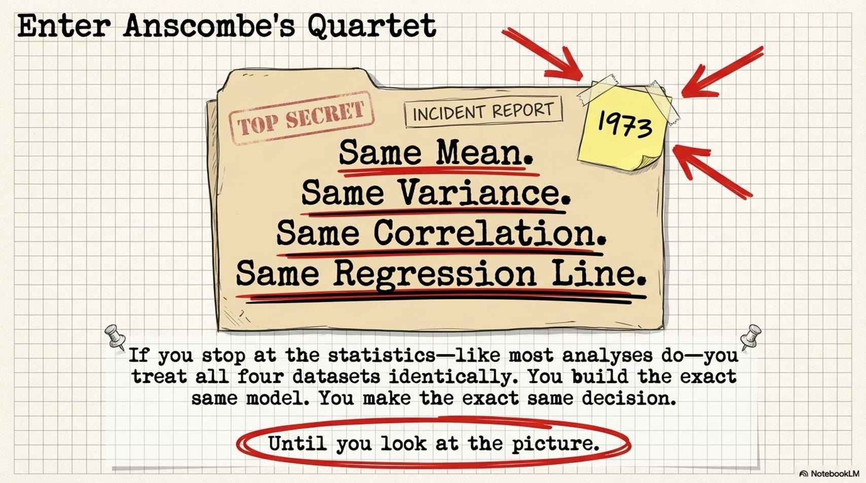
Published in 1973.
Half a century later, with dashboards generating auto-insights and AI tools summarizing datasets before you’ve seen a single plot, this lesson is more relevant than ever.
This is the walkthrough.
Four numbers. All identical. Here’s what each one actually measures.
When we say Anscombe’s four datasets have “identical statistics,” we mean four specific numbers match across all of them.
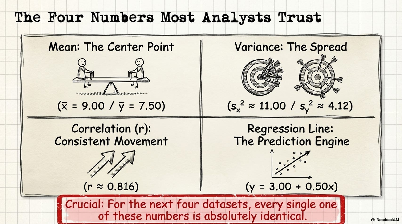
Here’s what each one measures - and more importantly, what it doesn’t.
Mean
Add up all your values. Divide by how many.
That’s the center point of your data.
In your work: An average CTR of 4.2% doesn’t tell you whether most campaigns cluster near 4% or whether half hit 1% and half hit 8%. It tells you the middle - and only the middle.
Formula: x̄ = (x₁ + x₂ + ... + xₙ) ÷ n - All four Anscombe datasets: mean X = 9.00, mean Y = 7.50.
Variance
For each data point, measure how far it sits from the mean. Square those distances. Average them.
That’s how spread out your data is around that center point.
In your work: If your average customer spends $50, variance tells you whether most customers actually spend near $50 (low variance - the average means something) or whether some spend $5 and some spend $300 (high variance - the average describes almost nobody).
Formula: s² = Σ(xᵢ − x̄)² ÷ (n − 1) - All four Anscombe datasets: variance X ≈ 11.00, variance Y ≈ 4.12.
Correlation coefficient (r)
How consistently X and Y move together, on a scale from −1 to +1.
Zero means no relationship. +1 means perfect lockstep. −1 means perfectly opposite.
In your work: r = 0.816 means “when one variable goes up, the other tends to go up too - and that relationship is strong and fairly consistent.” Strong enough to build a model on. Strong enough to shift a budget.
Formula: r = Σ[(xᵢ − x̄)(yᵢ − ȳ)] ÷ [(n−1) · sₓ · sᵧ] - All four Anscombe datasets: r ≈ 0.816.
Regression line
The formula for your trend line - your prediction engine.
The slope (b₁) tells you how much Y changes for every one-unit increase in X. The intercept (b₀) is where the line starts when X equals zero.
In your work: y = 3.00 + 0.50x means for every additional $1,000 in ad spend, you’d predict 500 more conversions plus a baseline of 3. This is the number most analysts hand to someone building a forecast.
Formula: y = b₀ + b₁x, where b₁ = r · (sᵧ ÷ sₓ) and b₀ = ȳ − b₁ · x̄ - All four Anscombe datasets produce the exact same equation.
Same mean. Same variance. Same correlation. Same regression line.
If you stopped at the statistics - and a lot of analyses do - you’d treat all four datasets identically. Same model. Same forecast. Same decision.
Then you’d look at the plots.
Four patterns. Four places you’ve seen this.
Dataset I - When the statistics are actually right.
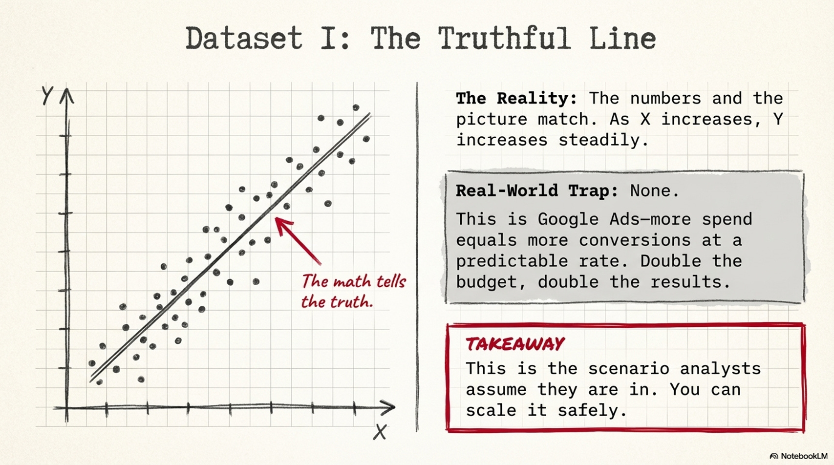
The plot: a clean diagonal. As X increases, Y increases steadily. The trend line fits.
Real-world version:
Google Ads spend vs. conversions tracked monthly. More spend, more conversions, at a consistent rate. The scatter looks exactly like this.
What this means:
The statistics are telling the truth. Forecast with confidence - double the budget, roughly double the results. Scale it.
This is also the exception, not the rule. Every other dataset in Anscombe’s Quartet has these exact same statistics - and none of them support the same forecast, the same model, or the same decision. The only way to know which one you’re actually looking at is to look.
Dataset II - The curve your model will never find.
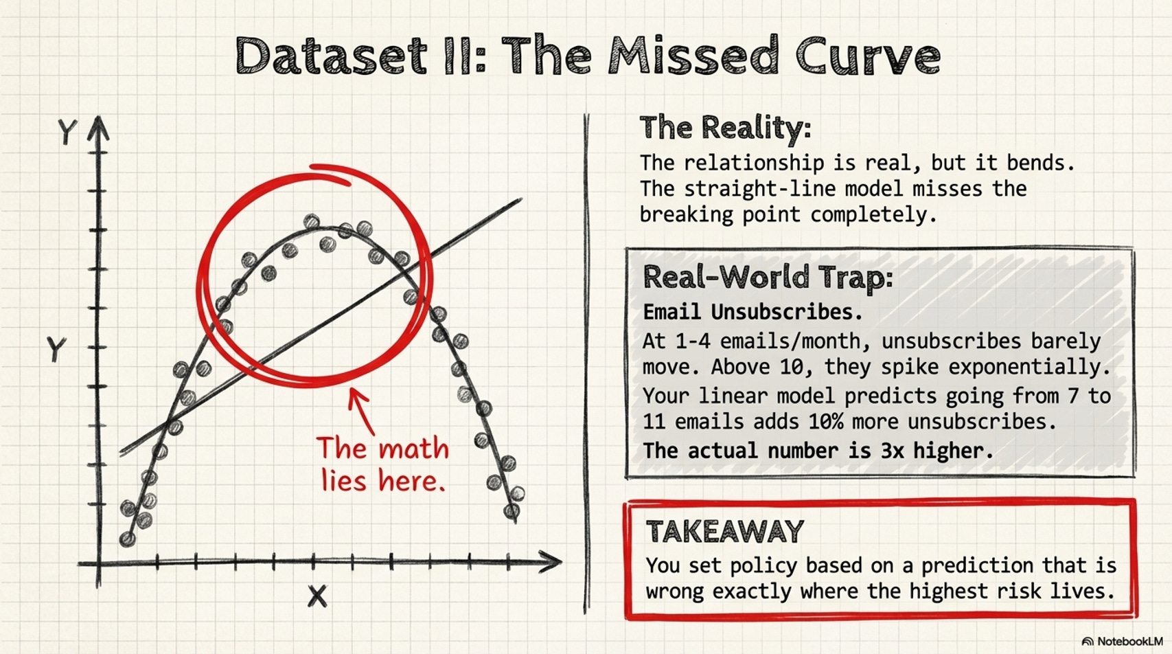
The plot: a smooth arc. The relationship is real - but it bends. This is a non-linear relationship: the change in Y per unit of X is not constant across the full range of values. It accelerates.
Real-world version:
Email send frequency vs. unsubscribe rate. At 1–4 emails per month, unsubscribes barely move. At 6–8, they start climbing. Above 10 per month, they spike - not gradually, but sharply.
The correlation and regression line describe this as a “moderate positive relationship.” They don’t show you the threshold - the frequency above which damage stops being manageable and starts accelerating. Your linear model predicts that going from 7 to 11 emails adds 10% more unsubscribes. The actual number is closer to 3×.
What this means:
You set your email cadence based on predictions that are wrong at exactly the frequencies that matter most. The model isn’t off by a small margin - it’s off in a way that shapes policy.
Dataset III - The one data point running everything.
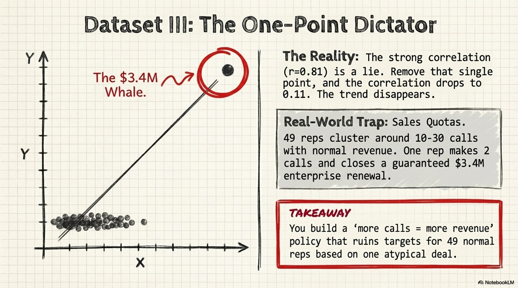
The plot: mostly linear - except for one extreme value, circled, pulling the regression line toward it.
Real-world version:
Sales CRM data - calls made per quarter vs. revenue closed. r = 0.81. “More calls equals more revenue.” A minimum call-volume policy gets written.
The scatter: 49 reps clustered between 10–30 calls and $50K–$200K in closed revenue. One enterprise account manager made 2 calls and closed a $3.4M renewal that was never at risk. Remove that one data point: r drops to 0.11. The “strong correlation” essentially disappears.
What this means:
You built a sales policy around a pattern that only applies to one atypical deal. Your best reps resent a quota that has no relationship to how their accounts actually close. The metric you’re tracking doesn’t predict the outcome you care about.
Dataset IV - The correlation that doesn’t actually exist.
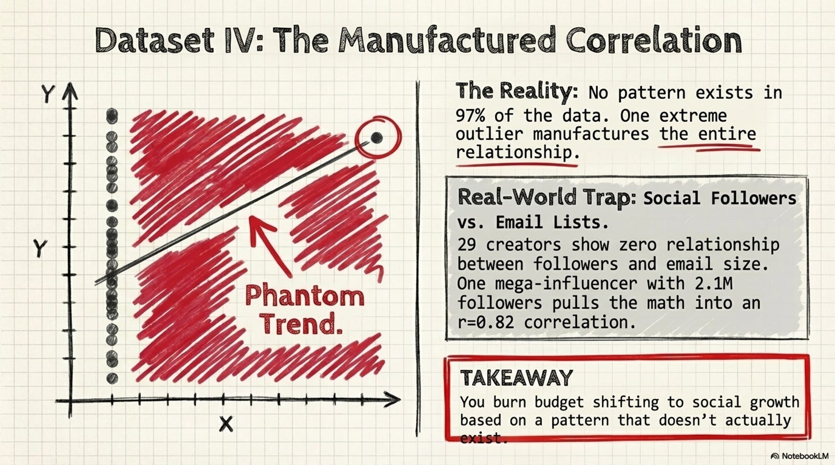
The plot: all points stacked at a single X value. One outlier far to the right, alone, manufacturing the entire correlation.
Real-world version:
A marketing analyst studies whether social media followers predict email list size across 30 content creators. r = 0.82. Strong signal. Budget shifts toward social growth, expecting email subscribers to follow.
The scatter: 29 creators between 5K–80K followers and 1K–15K email subscribers - no clear pattern. One creator with 2.1M followers and 180K email subscribers, sitting alone at the far right. Remove that one account: r = 0.09. No relationship.
What this means:
You spend a quarter investing in social growth expecting email to follow. It doesn’t - because the correlation was manufactured by one outlier. The decision was built on a pattern that didn’t exist for 97% of the data it claimed to describe.
The check worth running before every new dataset.
A few situations where you especially want to look before you calculate:
Your dataset has one record that’s dramatically larger or smaller than everything else
The relationship you’re modeling has a real-world reason to bend - pricing, frequency, diminishing returns, response thresholds
Your correlation looks strong but the sample is small
Almost every value in a variable is the same, with one or two exceptions
This is the prompt to save. Run it before you trust summary statistics on anything new:
I have a dataset I’m about to analyze. Before I run summary statistics or build a model, I want to understand its shape.

Here is the data: [paste or attach your data]

Please:

1. Generate a scatter plot or distribution chart for each numeric variable pair
2. Flag any curves or nonlinear patterns that a straight-line model would miss
3. Identify any extreme values that may be disproportionately influencing the result
4. Note if any variable has almost no variation except for one or two extreme cases
5. Summarize in plain language what I should know before I run correlations or regression on this data
This takes about 5 minutes on a new dataset.
It can help you catch things the statistics alone wouldn’t have surfaced.
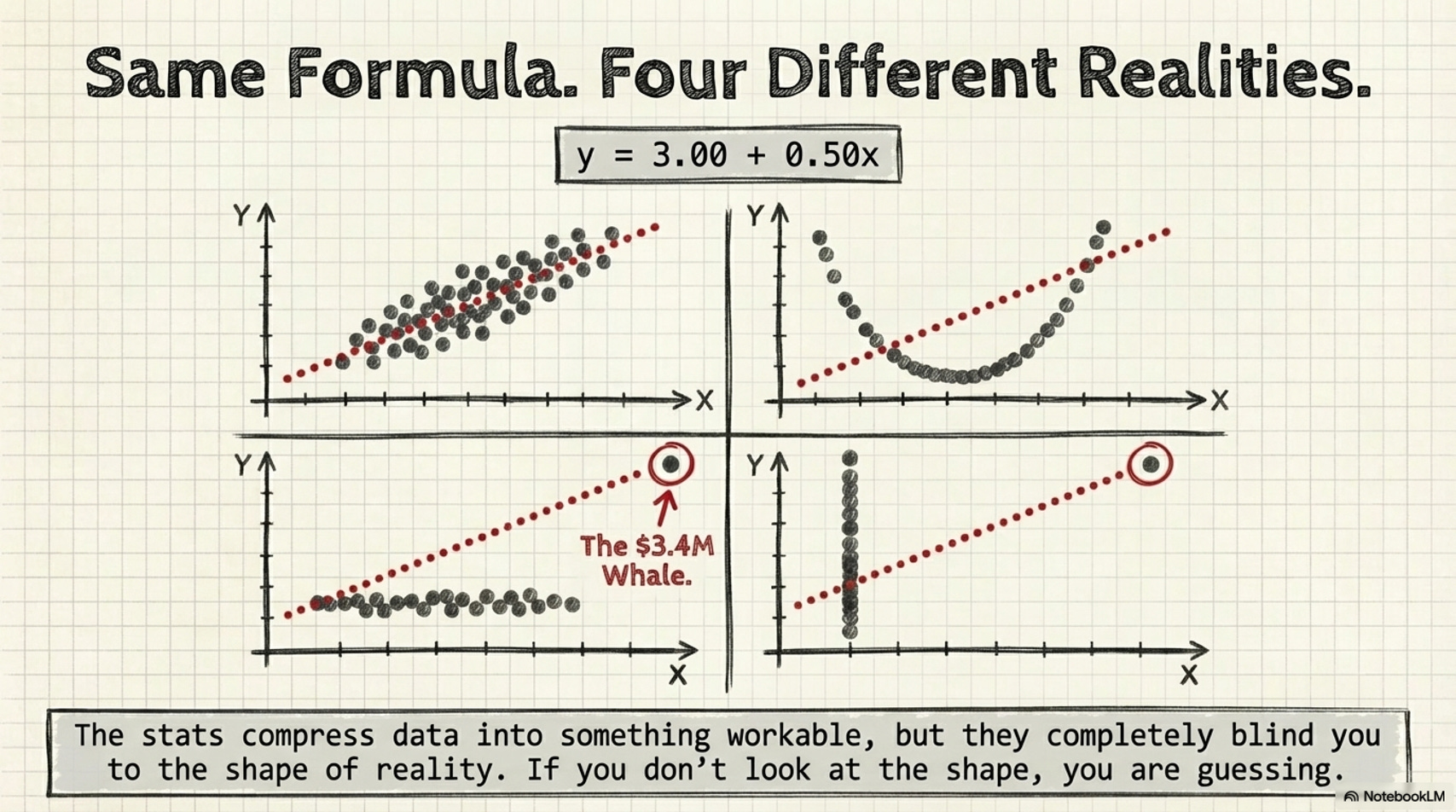
Summary statistics aren’t the problem.
Mean, variance, correlation, regression line - they do their job in most analyses. They compress data into something workable, and most of the time that’s exactly what you need.
The word is “most.”
There are specific situations where the shape of your data changes the decision entirely - the right model, the right forecast, the right strategy. That shape is invisible in the numbers. It only shows up in the picture.
Plot before you calculate.
Or at minimum, plot while you calculate. Once it’s a habit, it’s 10 minutes.
Once you’ve been caught by Dataset III or Dataset IV in a real analysis, you won’t skip it again.
Run it yourself - with Claude.
Reading about Anscombe’s Quartet lands at about 20% of what you get from actually running through it. Here’s the exercise.
Start with the data and statistics:
Generate Anscombe’s Quartet as a table - all four datasets (I, II, III, IV)
with X and Y values side by side. Then calculate and display the mean, variance,
correlation coefficient, and regression line formula for each dataset.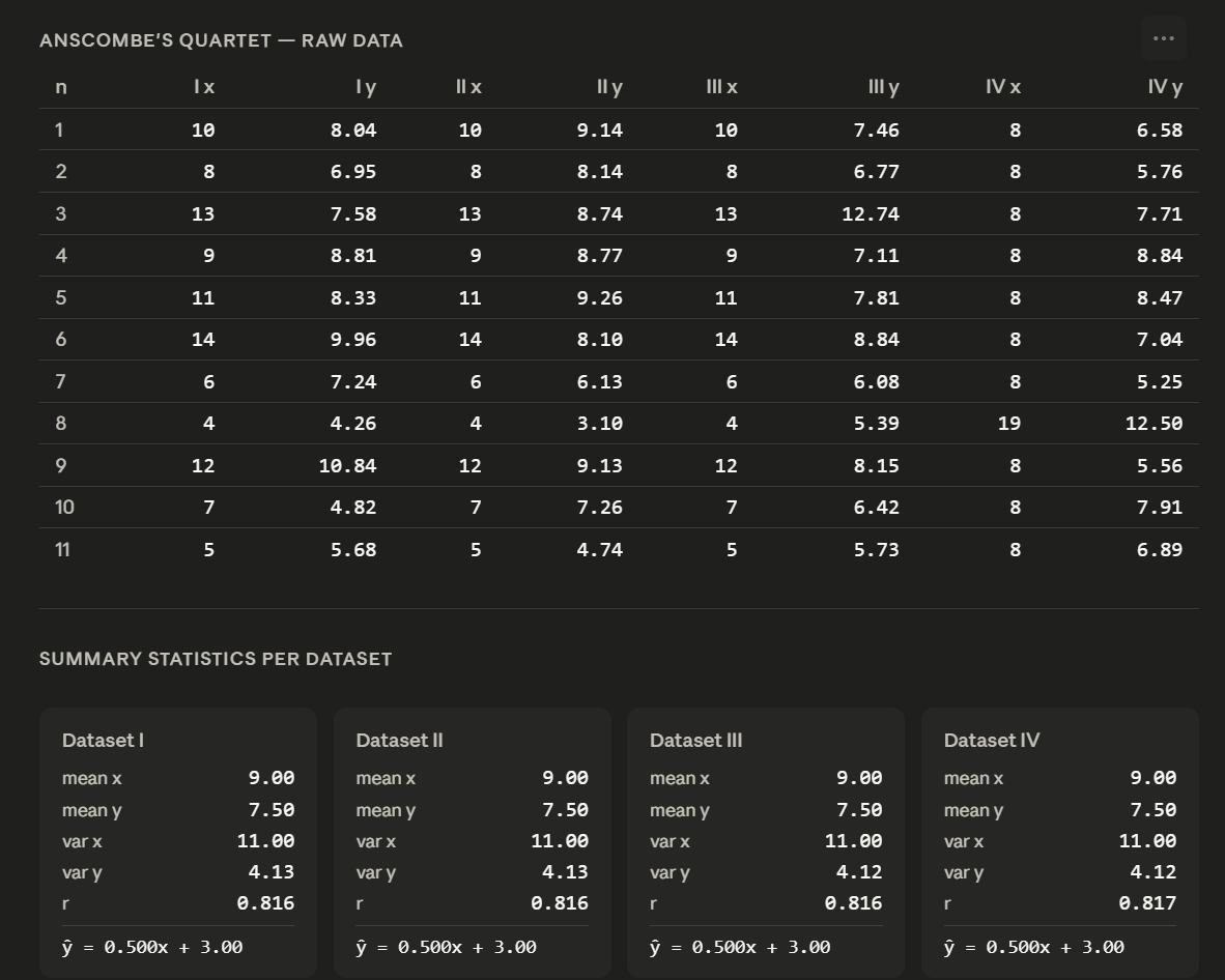
Sit with the output. The four datasets will look statistically identical. That’s the point.
Now ask for the visualization:
Create a 2×2 scatter plot of Anscombe’s Quartet using the data you just generated.
Label each dataset clearly. Add the regression line to each plot. Use a clean,
minimal style - white background, labeled axes, clear titles for each panel.
Watch what happens. Same statistics. Four different shapes.
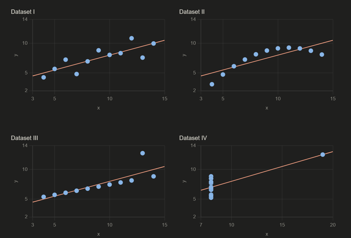
The regression line fits Dataset I. It misleads in Dataset II. It’s being dragged in Dataset III. In Dataset IV, it doesn’t describe a real relationship at all.
If you’re already working in Python, R, or Tableau, a scatter matrix does the same job. The Claude prompts here are the faster path when you’re starting from raw data and want to understand the shape before you’ve decided which tool to reach for.
If you’re teaching this: the exercise is the lesson.
Let students run the prompts before you explain what Anscombe’s Quartet is. The discovery moment does more than the definition.
Teach Data with AI is where I write about real analysis workflows, hands-on exercises worth doing, and the AI prompts I’m actually using in my data work. If this kind of practical approach is what you’ve been looking for, subscribe here.